38 pivot table multiple row labels
How to Filter Multiple Values in Pivot Table - Excel Tutorial When we click OK, we will have only LeBron James selected in our Pivot Table:. Filter with Slicers. Another way to filter multiple values in Pivot Table is to use Slicers.We will create another Pivot Table with the same data. Then we will place player, team, and conference in rows fields and the sum of points, rebounds, assists in the values field. Pivot Table Label Filters Tips - Contextures Excel Tips Jun 22, 2022 · The item is immediately hidden in the pivot table. Quickly Hide All But a Few Items. You can use a similar technique to hide most of the items in the Row Labels or Column Labels. Select the pivot table items that you want to keep visible; Right-click on one of the selected items; In the pop-up menu, click Filter, then click Keep Only Selected ...
How to add multiple fields into a pivot table in Excel? Step 1 At first, we must create a sample data for creating pivot table as shown in the below screenshot. Step 2 Now, select the data range from A1:J19. Click on the Insert tab on the tool bar ribbon and then select pivot table option to insert pivot table for the selected data range. Refer to the below screenshot for the same. Step 3

Pivot table multiple row labels
How to add side by side rows in excel pivot table - AnswerTabs To display more pivot table rows side by side, you need to turn on the Classic PivotTable layout and modify Field settings. For example will be used the following table: You have to right-click on pivot table and choose the PivotTable options. Then swich to Display tab and turn on Classic PivotTable layout: Pivot table - Wikipedia Row labels are used to apply a filter to one or more rows that have to be shown in the pivot table. For instance, if the "Salesperson" field is dragged on this area then the other output table constructed will have values from the column "Salesperson", i.e. , one will have a number of rows equal to the number of "Sales Person". Automatic Row And Column Pivot Table Labels - How To Excel At Excel Select the data set you want to use for your table The first thing to do is put your cursor somewhere in your data list Select the Insert Tab Hit Pivot Table icon Next select Pivot Table option Select a table or range option Select to put your Table on a New Worksheet or on the current one, for this tutorial select the first option Click Ok
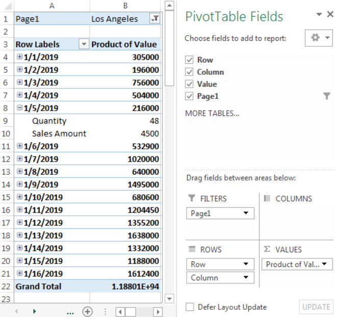
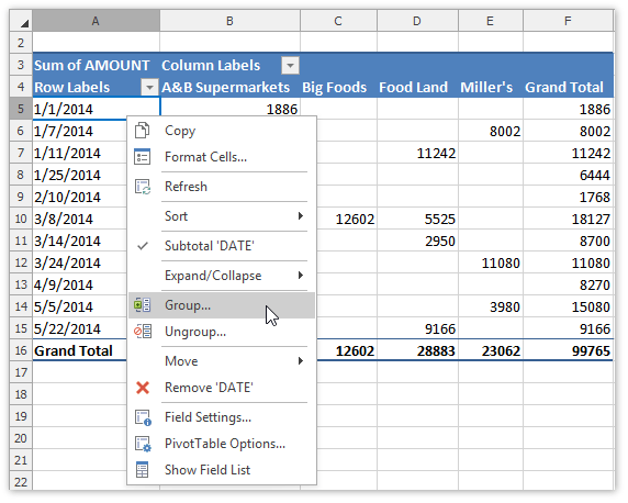
Pivot table multiple row labels. Excel Pivot Table Report Filter Tips and Tricks Jul 14, 2022 · To enable the grouping command, you’ll temporarily move the Report Filter field to the Row Labels area. In the screen shot below, the OrderDate field is being dragged to the Row Labels area, in the PivotTable fields pane. Then, right-click on the field in the pivot table, and click Group. Select the Grouping options that you want, and click OK How to repeat row labels for group in pivot table? - ExtendOffice Except repeating the row labels for the entire pivot table, you can also apply the feature to a specific field in the pivot table only. 1. Firstly, you need to expand the row labels as outline form as above steps shows, and click one row label which you want to repeat in your pivot table. 2. Excel: How to Apply Multiple Filters to Pivot Table at Once Example: Apply Multiple Filters to Excel Pivot Table. Suppose we have the following pivot table in Excel that shows the total sales of various products: Now suppose we click the dropdown arrow next to Row Labels, then click Label Filters, then click Contains: And suppose we choose to filter for rows that contain "shirt" in the row label: Apply Multiple Filters on a Pivot Field - Excel Pivot Tables Right-click any cell in the pivot table, and click PivotTable Options. Click the Totals & Filters tab. Under Filters, add a check mark to 'Allow multiple filters per field.'. Click OK. Now you can apply both a Label filter and a Value filter to the OrderMth field, and both will be retained. In the screen shot below, both the Label filter ...
Pivot Table Multiple Row Labels? [SOLVED] - excelforum.com Is it possible to have two Row Labels showing in a Pivot Table, instead of one showing as a sub-category of the other. I have a spreadsheet that shows the status (Design, Development, Testing, Live), owner and engineer for software. I currently have to have two separate pivot tables: 1) showing count of software in each status for each owner. Excel Pivot Table Multiple Consolidation Ranges Jul 25, 2022 · Pivot Tables > Create > Multiple Sources Pivot Table Multiple Consolidation Ranges. Create a Pivot Table using data from different sheets in a workbook, or from different workbooks, if those tables have identical column structures. Also, see alternatives to multiple consolidation ranges, by using Power Query or a Union Query. How to filter a pivot table with multiple filters - Exceljet To enable multiple filters per field, we need to change a setting in the pivot table options. Right-click in the pivot table and select PivotTable Options from the menu. then navigate to the Totals & Filters tab. There, under Filters, enable "allow multiple filters per field". Back in our pivot table, let's enable the Value Filter again ... Design the layout and format of a PivotTable After creating a PivotTable and adding the fields that you want to analyze, you may want to enhance the report layout and format to make the data easier to read and scan for details. To change the layout of a PivotTable, you can change the PivotTable form and the way that fields, columns, rows, subtotals, empty cells and lines are displayed.
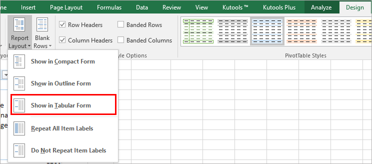
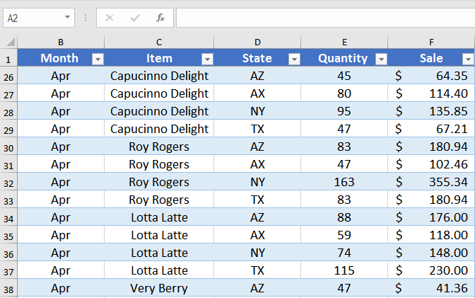
How to make row labels on same line in pivot table in excel #ExcelMaster, #PivotTable, #ExcelHow to make row labels on same line in pivot table in excelHow to show multiple rows in pivot table in excel How to make row labels on same line in pivot table? Make row labels on same line with setting the layout form in pivot table. As we all know, the pivot table has several layout form, the tabular form may help us to put the row labels next to each other. Please do as follows: 1. Click any cell in your pivot table, and the PivotTable Tools tab will be displayed. 2. Multi-level Pivot Table in Excel (Easy Tutorial) Multiple Row Fields First, insert a pivot table. Next, drag the following fields to the different areas. 1. Category field and Country field to the Rows area. 2. Amount field to the Values area. Below you can find the multi-level pivot table. Multiple Value Fields First, insert a pivot table. Next, drag the following fields to the different areas. Duplicate Items Appear in Pivot Table - Excel Pivot Tables Follow these steps to add a new field: Insert a new column in the source data, with the heading CityName. In Row 2 of the new column, enter the formula =TRIM (C2). Copy the formula down to the last row of data in the source table. If the source data is stored in an Excel Table, the formula should copy down automatically. Refresh the pivot table
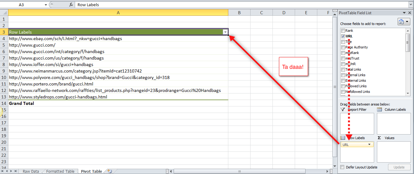
Pivot table row labels in separate columns • AuditExcel.co.za
PivotTable.RowFields property (Excel) | Microsoft Learn Example. This example adds the PivotTable report's row field names to a list on a new worksheet. VB. Set nwSheet = Worksheets.Add nwSheet.Activate Set pvtTable = Worksheets ("Sheet2").Range ("A1").PivotTable rw = 0 For Each pvtField In pvtTable.RowFields rw = rw + 1 nwSheet.Cells (rw, 1).Value = pvtField.Name Next pvtField.
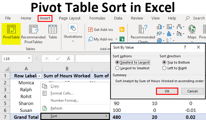
Pivot Table Sort in Excel | How to Sort Pivot Table Columns ...
Multiple row labels on one row in Pivot table - MrExcel Message Board I figured it out - Right click on your pivot table and choose pivot table options/display. Click on "Classic PivotTable layout" Then click on where it is subtotaling your row label and uncheck the subtotal option. D dudeshane0 New Member Joined Oct 23, 2014 Messages 1 Jan 19, 2015 #6 Gerald Higgins said:
Excel Pivot Tables Explained • My Online Training Hub
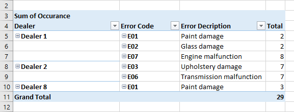
Pivot Table Row Labels In the Same Line - Beat Excel! Then navigate to "Layout & Print" tab and click on "Show item in tabular form" option. Do this procedure also for "Dealer" field and your table will look like this: If you also want dealer names to repeat on each row, reopen "Dealer field settings and check "Repear item labels" option in "Layout & Print" tab.

Changing Order of Row Labels in Pivot Table
Pivot Table from Multiple Sheets | How to Create a Pivot Table? Filter in Pivot Table Filter In Pivot Table By right-clicking on the pivot table, we can access the pivot table filter option. Another approach is to use the filter options available in the pivot table fields. read more; Delete the Pivot Table Delete The Pivot Table To delete a pivot table in Excel, you must first select it. Then go to the ...

Excel Pivot Table Multiple Consolidation Ranges
Pivot table when same record appears multiple times However, if I create pivot table to summarize the count by restaurant type I'll get an inaccurate result. Row Labels Count of Restaurant Type Diner 1 Fast Food 4 Grand Total 5 This is an inaccurate count since the total number of Fast Food Restaurant Type should be 1 and the total number of Diner Restaurant Type should be 1.

How to make row labels on same line in pivot table?
Sort multiple row label in pivot table - Microsoft Community Hi All. Could anybody suggest how to sort the pivot table row field data if it contains multiple headers :-. for example : In below given example I want to sort the data of column B in asending order , but when I am applying sorting here it is not sorting. Thanks in advance for your suggestion. This thread is locked.

Making Report Layout Changes | Customizing an Excel 2013 ...
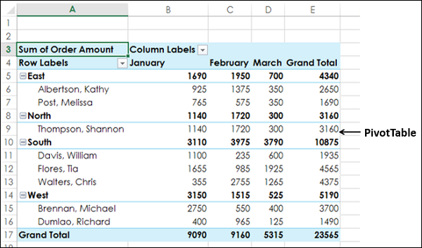
Make an Excel PivotTable with multiple or nested rows Make an Excel PivotTable with multiple or nested rows 23 October 2017 A list with groupings (like Product Type, Country, Region or Staff pay level) can become a nested PivotTable. The sub-totals are created with + - signs to show/hide the groupings. We're using the same source list as in our Basic PivotTable and Two-dimensional PivotTable examples.
How to Filter Data in a Pivot Table in Excel
Pivot table row labels in separate columns • AuditExcel.co.za Our preference is rather that the pivot tables are shown in tabular form (all columns separated and next to each other). You can do this by changing the report format. So when you click in the Pivot Table and click on the DESIGN tab one of the options is the Report Layout. Click on this and change it to Tabular form.

Repeat all item labels in Pivot Table (aka Fill in the blanks ...
Pivot table row labels side by side - Excel Tutorial - OfficeTuts Excel You can copy the following table and paste it into your worksheet as Match Destination Formatting. Now, let's create a pivot table ( Insert >> Tables >> Pivot Table) and check all the values in Pivot Table Fields. Fields should look like this. Right-click inside a pivot table and choose PivotTable Options…. Check data as shown on the image below.
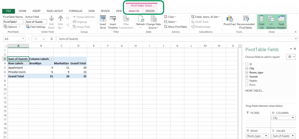
The Pivot table tools ribbon in Excel
Pivot Table row labels in separate columns - YouTube 00:00 Pivot table has multiple fields in one column00:15 Change the Pivot Table field to appear in their own columns00:30 Each column is one Pivot Table fiel...
How to make row labels on same line in pivot table?
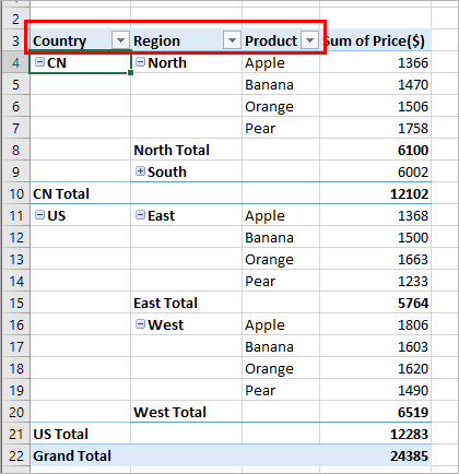
Excel Pivot Table with nested rows | Basic Excel Tutorial The table on the left shows a multi-level pivot table with the results of the selected fields. This table shows summarized data with customers' names and the products bought. Adding fields to the row label automatically groups your PivotTable based on customers' names as Level one followed by products grouped as level 2.

Excel: How to Apply Multiple Filters to Pivot Table at Once ...
Multi-row and Multi-column Pivot Table - Excel Start Click OK Once the pivot table sheet is created, just like in the previous example, drag the Category and the Product to the Rows section and the Sales Value to the Values section to get the same Multi-Row pivot table we did in the previous example. Next we want to add a column. We will add the Date to the Column section by dragging the field.

Permanently Tabulate Pivot Table Report & Repeat All Item ...
How to Move Pivot Table Labels - Contextures Excel Tips Jul 12, 2021 · Move Pivot Table Labels. This short video shows 3 ways to manually move the labels in a pivot table, and the written instructions are below the video. Drag a Label. Use Menu Commands. Type over a Label. Drag Labels to New Position. To move a pivot table label to a different position in the list, you can drag it: Click on the label that you want ...
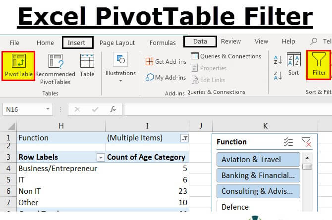
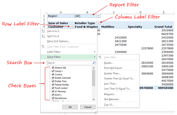
Pivot Table Filter in Excel | How to Filter Data in a Pivot ...
multiple fields as row labels on the same level in pivot table Excel ... multiple fields as row labels on the same level in pivot table Excel 2016 I am using Excel 2016. I have data that lists product models along with relevant data and also production volumes by month. Part of the relevant data are about 5 common part columns with the part # that applies to each model under the appropriate column.

Pivot Tables in Excel - Earn & Excel
Automatic Row And Column Pivot Table Labels - How To Excel At Excel Select the data set you want to use for your table The first thing to do is put your cursor somewhere in your data list Select the Insert Tab Hit Pivot Table icon Next select Pivot Table option Select a table or range option Select to put your Table on a New Worksheet or on the current one, for this tutorial select the first option Click Ok

How to Filter Data in a Pivot Table in Excel
Pivot table - Wikipedia Row labels are used to apply a filter to one or more rows that have to be shown in the pivot table. For instance, if the "Salesperson" field is dragged on this area then the other output table constructed will have values from the column "Salesperson", i.e. , one will have a number of rows equal to the number of "Sales Person".
How to make row labels on same line in pivot table?
How to add side by side rows in excel pivot table - AnswerTabs To display more pivot table rows side by side, you need to turn on the Classic PivotTable layout and modify Field settings. For example will be used the following table: You have to right-click on pivot table and choose the PivotTable options. Then swich to Display tab and turn on Classic PivotTable layout:

Pivot table row labels side by side – Excel Tutorial
Excel Pivot Tables - Sorting Data
Pivot Table shows row labels instead of field name

Pivot table row labels in separate columns • AuditExcel.co.za

Pivot Table Row Labels In the Same Line - Beat Excel!

Problems with multiple text fields in a Pivot Table ...
How To Manage Big Data With Pivot Tables
How to Create a Pivot Table from Multiple Worksheets | Excelchat
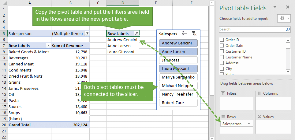
3 Ways to Display (Multiple Items) Filter Criteria in a Pivot ...

image122.png

Permanently Tabulate Pivot Table Report & Repeat All Item ...

How to make row labels on same line in pivot table?

Excel Pivot Table with multiple columns of data and each data ...

Excel: How to Apply Multiple Filters to Pivot Table at Once ...
Instructions for Sorting a Pivot Table by Two Columns | Excelchat
Multi-level Pivot Table in Excel (Easy Tutorial)

Pivot table row labels in separate columns • AuditExcel.co.za
Group Items in a Pivot Table | DevExpress End-User Documentation
MS Excel 2013: Display the fields in the Values Section in ...
Pivot table row labels side by side – Excel Tutorial
Instructions for Sorting a Pivot Table by Two Columns | Excelchat
Post a Comment for "38 pivot table multiple row labels"